---

每日一句正能量

内心承载使命之人，可在平凡中孕育伟大，也能在逆旅中成就不凡。
有使命的人，日常的平凡工作也有了意义感（孕育伟大）；遭遇逆境也能转化为养分（逆旅中成就不凡）。沉淀自己不是为了独善其身，而是为了承载更大的东西。

摘要

摘要：本文深入探讨长短期记忆网络（LSTM）在嵌入式边缘设备上的轻量化部署与优化实践。从LSTM门控单元的数学原理出发，系统分析状态缓存机制的设计策略、INT8量化与结构化剪枝的压缩方法，以及算子融合与内存优化的工程技巧。结合STM32、ESP32、RK3588、Jetson等典型边缘平台的性能对比，为工业预测维护、智能传感等场景的端侧AI部署提供完整技术方案。

---

一、LSTM门控单元原理与数学基础

长短期记忆网络（Long Short-Term Memory, LSTM）通过引入门控机制解决了传统RNN的梯度消失问题，成为时序预测任务的首选架构。理解其内部结构是边缘优化的前提。

1.1 LSTM单元结构详解

LSTM的核心是一个记忆细胞（Cell State），配合三个门控单元共同控制信息的流动：

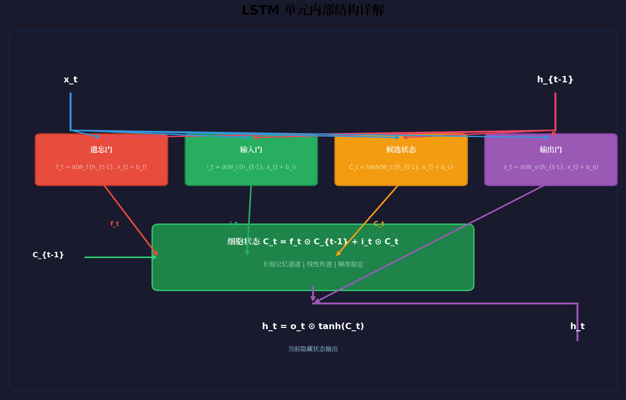
图1：LSTM单元内部结构详解

四个核心计算步骤：

$$\begin{array}{rl}\text{遗忘门: }& f_t=\sigma (W_f\cdot [h_{t-1},x_t]+b_f)\\ \text{输入门: }& i_t=\sigma (W_i\cdot [h_{t-1},x_t]+b_i)\\ \text{候选状态: }& {\tilde{C}}_t=\tanh (W_c\cdot [h_{t-1},x_t]+b_c)\\ \text{输出门: }& o_t=\sigma (W_o\cdot [h_{t-1},x_t]+b_o)\end{array}$$

状态更新：

$$\begin{array}{rl}{C}_t& =f_t\odot C_{t-1}+i_t\odot {\tilde{C}}_t\\ h_t& =o_t\odot \tanh (C_t)\end{array}$$

其中 $\odot$ 表示逐元素乘法（Hadamard积），$\sigma$ 为Sigmoid函数，输出范围 $(0,1)$，用于控制门的开闭程度；$\tanh$ 输出范围 $(-1,1)$，用于生成候选状态。

1.2 门控单元的工程意义

门控	功能	边缘优化要点
遗忘门 $f_t$	决定丢弃多少历史信息	初始化偏置为1.0，避免早期遗忘
输入门 $i_t$	控制新信息写入比例	与候选状态合并计算，减少内存访问
候选状态 ${\tilde{C}}_t$	生成新的候选记忆	使用tanh近似函数加速
输出门 $o_t$	决定输出多少当前记忆	可与最终输出合并计算

---

二、边缘设备LSTM部署架构

2.1 端到端数据流设计

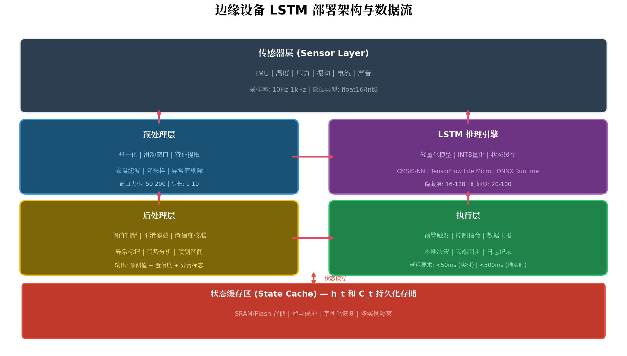
图2：边缘设备LSTM部署架构与数据流

边缘LSTM推理系统包含五个关键层次：

传感器层：采集原始时序数据（IMU、温度、压力、振动等），采样率通常为10Hz-1kHz。数据类型建议直接采集为float16或int16，减少后续转换开销。

预处理层：执行滑动窗口、归一化、滤波去噪。关键参数：

• 窗口大小：50-200个时间步（根据信号周期确定）
• 步长：1-10（步长=1时信息密度最高，但计算量最大）
• 归一化：使用训练集的均值和标准差，边缘端固定缩放因子

LSTM推理引擎：核心计算层，需针对目标平台选择推理框架：

• MCU级（STM32/ESP32）：CMSIS-NN、TensorFlow Lite Micro
• MPU级（RK3588/树莓派）：ONNX Runtime、Tengine
• GPU级（Jetson）：TensorRT、ONNX Runtime CUDA Execution Provider

后处理层：阈值判断、平滑滤波、置信度校准。输出通常包含预测值、异常标志和置信度。

执行层：触发预警、生成控制指令、上报云端。

2.2 状态缓存的核心挑战

LSTM是有状态（Stateful）模型，$h_t$ 和 $C_t$ 必须在时间步之间传递。边缘设备面临的挑战：

1. 内存限制：MCU的SRAM仅几十KB到几百KB
2. 掉电丢失：设备重启后状态丢失，影响预测连续性
3. 多实例隔离：同一设备运行多个LSTM实例时状态不能混淆
4. 实时性要求：状态读写不能阻塞推理流水线

---

三、状态缓存机制设计与实现

3.1 状态缓存架构

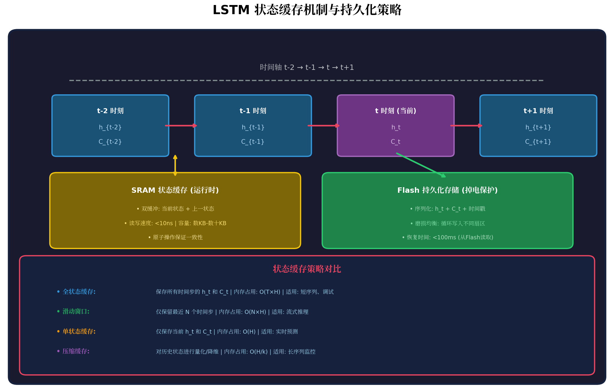
图3：LSTM状态缓存机制与持久化策略

SRAM运行时缓存：

• 采用双缓冲策略：当前状态 + 上一状态
• 读写速度 <10ns，适合高频访问
• 使用原子操作保证并发安全

Flash持久化存储：

• 序列化格式：[时间戳(4B)] [h_t(2H B)] [C_t(2H B)] [CRC(2B)]
• 磨损均衡：循环写入不同扇区，延长Flash寿命
• 恢复时间：<100ms（从Flash读取并反序列化）

3.2 状态缓存策略对比

策略	内存占用	适用场景	实现复杂度
全状态缓存	$O(T\times H)$	短序列调试、可视化	低
滑动窗口	$O(N\times H)$	流式推理、异常检测	中
单状态缓存	$O(H)$	实时预测、资源受限	低
压缩缓存	$O(H/k)$	长序列监控、历史回溯	高

推荐策略：对于大多数边缘预测场景，单状态缓存是最优选择——仅保存当前的 $h_t$ 和 $C_t$，内存占用最小，且满足实时推理需求。

3.3 状态缓存代码实现

// LSTM状态缓存结构体 (适用于嵌入式C/C++)
typedef struct {
    uint32_t timestamp;      // 时间戳
    uint16_t hidden_size;    // 隐藏层维度
    float*   cell_state;     // C_t 细胞状态
    float*   hidden_state;   // h_t 隐藏状态
    uint16_t crc;            // CRC校验
} LSTM_StateCache;

// SRAM运行时缓存 (双缓冲)
typedef struct {
    LSTM_StateCache buf[2];  // 双缓冲
    uint8_t active_idx;      // 当前活跃缓冲区
} LSTM_StateBuffer;

// 初始化状态缓存
int lstm_state_init(LSTM_StateBuffer* state, uint16_t hidden_size) {
    state->active_idx = 0;
    for (int i = 0; i < 2; i++) {
        state->buf[i].hidden_size = hidden_size;
        state->buf[i].cell_state = (float*)malloc(hidden_size * sizeof(float));
        state->buf[i].hidden_state = (float*)malloc(hidden_size * sizeof(float));
        if (!state->buf[i].cell_state || !state->buf[i].hidden_state) {
            return -1; // 内存分配失败
        }
        memset(state->buf[i].cell_state, 0, hidden_size * sizeof(float));
        memset(state->buf[i].hidden_state, 0, hidden_size * sizeof(float));
    }
    return 0;
}

// 读取当前状态 (用于推理输入)
void lstm_state_read(LSTM_StateBuffer* state, float** cell, float** hidden) {
    uint8_t idx = state->active_idx;
    *cell = state->buf[idx].cell_state;
    *hidden = state->buf[idx].hidden_state;
}

// 写入新状态 (推理完成后)
void lstm_state_write(LSTM_StateBuffer* state, float* new_cell, float* new_hidden) {
    uint8_t next_idx = 1 - state->active_idx;  // 切换缓冲区
    memcpy(state->buf[next_idx].cell_state, new_cell, 
           state->buf[next_idx].hidden_size * sizeof(float));
    memcpy(state->buf[next_idx].hidden_state, new_hidden,
           state->buf[next_idx].hidden_size * sizeof(float));
    state->active_idx = next_idx;  // 原子更新索引
}

// Flash持久化 (掉电保护)
int lstm_state_persist(LSTM_StateBuffer* state, uint32_t flash_addr) {
    uint8_t idx = state->active_idx;
    LSTM_StateCache* cache = &state->buf[idx];
    cache->timestamp = get_system_timestamp();
    cache->crc = calculate_crc16((uint8_t*)cache, 
                   sizeof(LSTM_StateCache) - sizeof(uint16_t));
    
    // 磨损均衡：循环写入
    static uint32_t write_offset = 0;
    uint32_t addr = flash_addr + write_offset;
    write_offset = (write_offset + sizeof(LSTM_StateCache)) % FLASH_SECTOR_SIZE;
    
    return flash_write(addr, (uint8_t*)cache, sizeof(LSTM_StateCache));
}

// 从Flash恢复状态
int lstm_state_restore(LSTM_StateBuffer* state, uint32_t flash_addr) {
    LSTM_StateCache temp;
    if (flash_read(flash_addr, (uint8_t*)&temp, sizeof(LSTM_StateCache)) != 0) {
        return -1;
    }
    
    // CRC校验
    uint16_t calc_crc = calculate_crc16((uint8_t*)&temp, 
                        sizeof(LSTM_StateCache) - sizeof(uint16_t));
    if (calc_crc != temp.crc) {
        return -2; // 数据损坏
    }
    
    // 恢复到活跃缓冲区
    uint8_t idx = state->active_idx;
    memcpy(state->buf[idx].cell_state, temp.cell_state, 
           temp.hidden_size * sizeof(float));
    memcpy(state->buf[idx].hidden_state, temp.hidden_state,
           temp.hidden_size * sizeof(float));
    
    return 0;
}

---

四、模型轻量化与量化压缩

4.1 轻量化策略全景

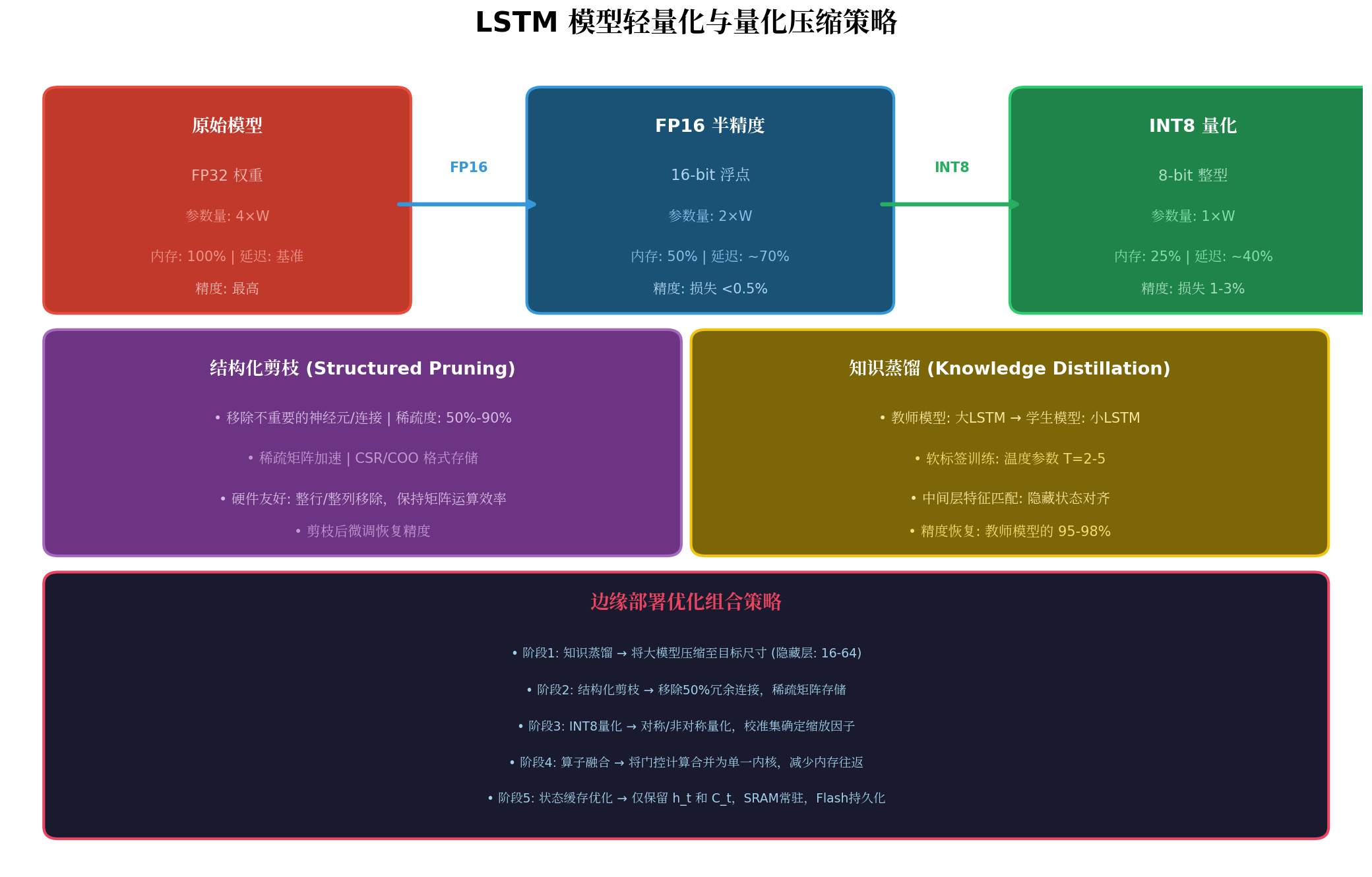
图4：LSTM模型轻量化与量化压缩策略

4.2 INT8对称量化实现

INT8量化是将FP32权重映射到8位整型的过程，核心公式：

$$\begin{array}{rl}{W}_{int8}& =\text{round}\left(\frac{W_{fp32}}{scale}\right)\\ scale& =\frac{\max (|W_{fp32}|)}{127}\end{array}$$

推理时的反量化：

$$y_{fp32}=scale\cdot (W_{int8}\cdot x_{int8})$$

LSTM INT8量化特殊处理：

// LSTM INT8量化推理核心 (CMSIS-NN风格)
#include "arm_nnfunctions.h"

typedef struct {
    int8_t*  weights;        // INT8权重
    int32_t* bias;           // INT32偏置 (累加用)
    int16_t  input_scale;    // 输入缩放因子
    int16_t  output_scale;   // 输出缩放因子
    int8_t   input_zero_point;   // 输入零点
    int8_t   output_zero_point;  // 输出零点
} LSTM_QuantParams;

// INT8 LSTM单步推理
void lstm_int8_step(
    const int8_t* input,           // 量化输入
    int8_t* hidden_state,          // 量化隐藏状态 (输入/输出)
    int8_t* cell_state,            // 量化细胞状态
    const LSTM_QuantParams* params,
    int16_t input_size,
    int16_t hidden_size)
{
    // 1. 反量化输入和隐藏状态到INT32 (用于累加)
    int32_t input_int32[INPUT_SIZE];
    int32_t hidden_int32[HIDDEN_SIZE];
    
    for (int i = 0; i < input_size; i++) {
        input_int32[i] = (int32_t)(input[i] - params->input_zero_point);
    }
    for (int i = 0; i < hidden_size; i++) {
        hidden_int32[i] = (int32_t)(hidden_state[i] - params->input_zero_point);
    }
    
    // 2. 合并矩阵乘法 (4门合并为1次GEMM)
    // 计算 [f_t, i_t, o_t, C_tilde] 的预激活值
    int32_t gate_preact[4 * HIDDEN_SIZE];
    
    // 使用CMSIS-NN的矩阵乘法
    arm_fully_connected_mat_q7_vec_q15_opt(
        input,                    // 输入向量
        params->weights,          // 合并权重 (4H x (input+hidden))
        input_size + hidden_size, // 输入维度
        4 * hidden_size,          // 输出维度
        0,                        // 偏置偏移
        1,                        // 输出偏移
        gate_preact,              // 输出
        NULL                      // 临时缓冲区
    );
    
    // 3. 激活函数 (INT8近似)
    for (int g = 0; g < 4; g++) {
        for (int h = 0; h < hidden_size; h++) {
            int idx = g * hidden_size + h;
            if (g < 3) {
                // Sigmoid: 使用查找表或分段线性近似
                gate_preact[idx] = sigmoid_int8_approx(gate_preact[idx]);
            } else {
                // Tanh: 使用查找表或分段线性近似
                gate_preact[idx] = tanh_int8_approx(gate_preact[idx]);
            }
        }
    }
    
    // 4. 门控计算与状态更新
    for (int h = 0; h < hidden_size; h++) {
        int32_t f = gate_preact[h];              // 遗忘门
        int32_t i = gate_preact[hidden_size + h]; // 输入门
        int32_t o = gate_preact[2*hidden_size + h]; // 输出门
        int32_t c_tilde = gate_preact[3*hidden_size + h]; // 候选状态
        
        // 细胞状态更新: C_t = f * C_{t-1} + i * C_tilde
        int32_t cell_int32 = (f * cell_state[h]) >> 7;  // 定点乘法
        cell_int32 += (i * c_tilde) >> 7;
        cell_state[h] = (int8_t)clamp(cell_int32, -127, 127);
        
        // 隐藏状态更新: h_t = o * tanh(C_t)
        int32_t tanh_cell = tanh_int8_approx(cell_state[h]);
        int32_t hidden_int32 = (o * tanh_cell) >> 7;
        hidden_state[h] = (int8_t)clamp(hidden_int32, -127, 127);
    }
}

// Sigmoid INT8查找表近似 (256 entry)
static const int8_t sigmoid_lut[256] = {
    0, 0, 0, 0, 0, 0, 0, 0, 0, 0, 0, 1, 1, 1, 1, 1,
    // ... 完整查找表
    126, 127, 127, 127, 127, 127, 127, 127, 127, 127, 127, 127, 127, 127, 127, 127
};

int8_t sigmoid_int8_approx(int32_t x) {
    // 将INT32映射到0-255索引
    int idx = (x + 128) >> 1;  // 缩放并偏移
    idx = clamp(idx, 0, 255);
    return sigmoid_lut[idx];
}

4.3 结构化剪枝

# PyTorch LSTM结构化剪枝示例
import torch
import torch.nn as nn
import torch.nn.utils.prune as prune

# 定义LSTM模型
class LSTM_Predictor(nn.Module):
    def __init__(self, input_size, hidden_size, num_layers):
        super().__init__()
        self.lstm = nn.LSTM(input_size, hidden_size, num_layers, 
                           batch_first=True)
        self.fc = nn.Linear(hidden_size, 1)
    
    def forward(self, x):
        lstm_out, _ = self.lstm(x)
        return self.fc(lstm_out[:, -1, :])

# 结构化剪枝：移除50%的隐藏单元
model = LSTM_Predictor(input_size=6, hidden_size=64, num_layers=1)

# 对LSTM权重矩阵进行结构化剪枝 (按行/列)
prune.ln_structured(model.lstm, name='weight_ih_l0', 
                    amount=0.5, n=1, dim=0)  # dim=0: 按行剪枝
prune.ln_structured(model.lstm, name='weight_hh_l0', 
                    amount=0.5, n=1, dim=0)

# 剪枝后微调恢复精度
# 注意：剪枝后需要重新训练或微调

---

五、门控单元算子融合优化

5.1 计算流程优化

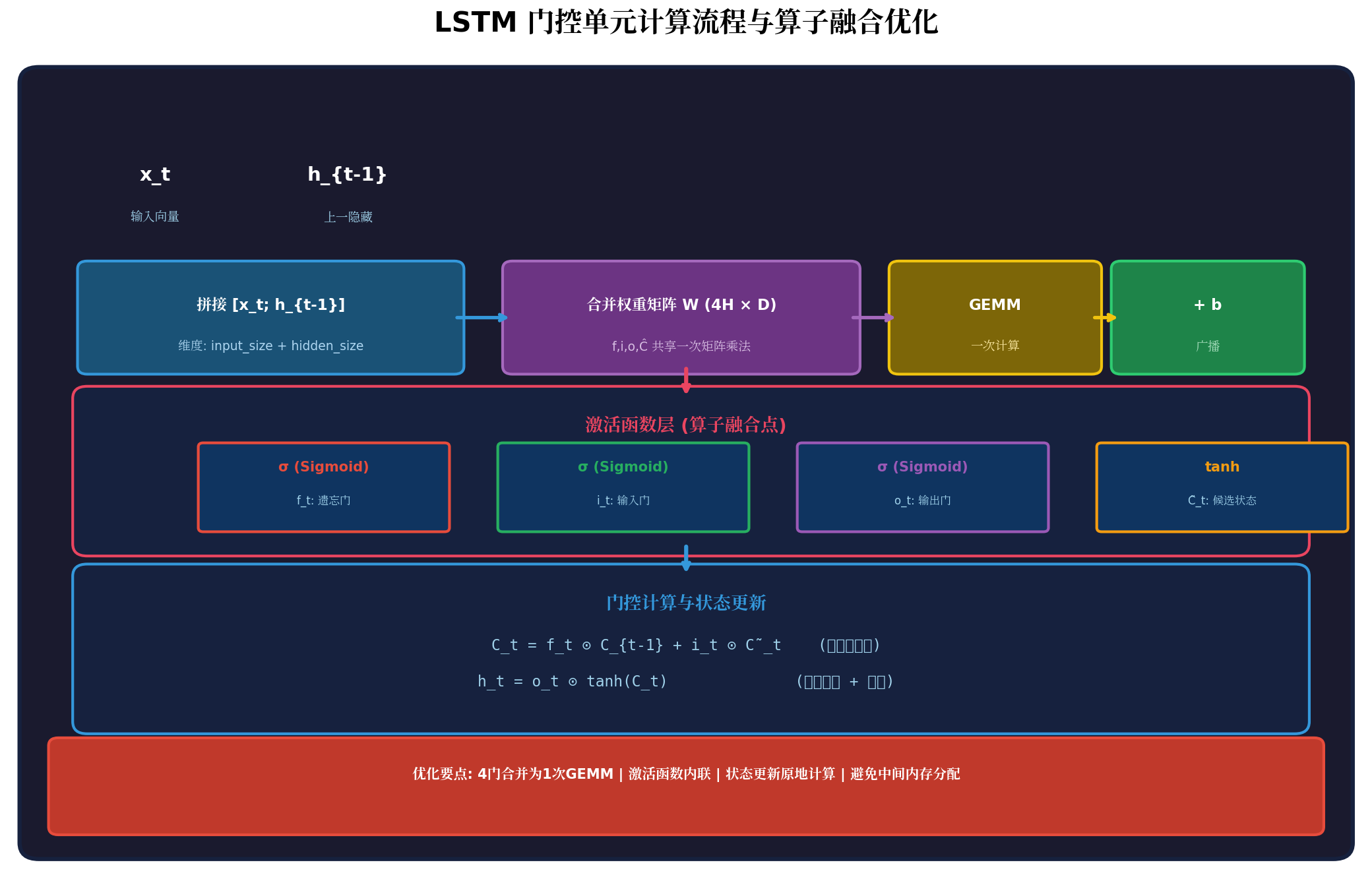
图5：LSTM门控单元计算流程与算子融合优化

标准LSTM的计算瓶颈：

• 4次独立的矩阵-向量乘法（GEMV）
• 4次独立的偏置加法
• 4次独立的激活函数
• 多次中间结果内存分配

优化后的融合计算：

// 融合LSTM单步推理 (C++实现)
void lstm_fused_step(
    const float* input,      // 输入 x_t
    float* hidden_state,     // h_{t-1} / h_t
    float* cell_state,       // C_{t-1} / C_t
    const float* weights,    // 合并权重 [W_f; W_i; W_o; W_c] (4H x D)
    const float* bias,       // 合并偏置 [b_f; b_i; b_o; b_c]
    int input_size,
    int hidden_size)
{
    const int total_input = input_size + hidden_size;
    const int gate_size = 4 * hidden_size;
    
    // 拼接输入: [x_t; h_{t-1}]
    float concat[total_input];
    memcpy(concat, input, input_size * sizeof(float));
    memcpy(concat + input_size, hidden_state, hidden_size * sizeof(float));
    
    // 一次矩阵乘法计算所有门 (GEMM融合)
    float gate_preact[gate_size];
    gemm_fused(gate_preact, weights, concat, gate_size, total_input, bias);
    
    // 激活函数内联 (避免函数调用开销)
    for (int g = 0; g < 3; g++) {  // f, i, o: sigmoid
        for (int h = 0; h < hidden_size; h++) {
            gate_preact[g * hidden_size + h] = 
                sigmoid_fast(gate_preact[g * hidden_size + h]);
        }
    }
    // c_tilde: tanh
    for (int h = 0; h < hidden_size; h++) {
        gate_preact[3 * hidden_size + h] = 
            tanh_fast(gate_preact[3 * hidden_size + h]);
    }
    
    // 状态更新 (原地计算，避免额外内存分配)
    for (int h = 0; h < hidden_size; h++) {
        float f = gate_preact[h];
        float i = gate_preact[hidden_size + h];
        float o = gate_preact[2 * hidden_size + h];
        float c_tilde = gate_preact[3 * hidden_size + h];
        
        // C_t = f * C_{t-1} + i * c_tilde
        cell_state[h] = f * cell_state[h] + i * c_tilde;
        
        // h_t = o * tanh(C_t)
        hidden_state[h] = o * tanh_fast(cell_state[h]);
    }
}

// 快速Sigmoid近似 (避免exp计算)
inline float sigmoid_fast(float x) {
    // 分段线性近似或使用tanh
    return 0.5f * (1.0f + tanh_fast(0.5f * x));
}

// 快速Tanh近似 (多项式或查找表)
inline float tanh_fast(float x) {
    // 使用Pade近似或硬tanh
    float x2 = x * x;
    return x * (27.0f + x2) / (27.0f + 9.0f * x2);
}

5.2 内存布局优化

// 优化后的权重内存布局 (SoA - Structure of Arrays)
// 原始布局: [W_f][W_i][W_o][W_c] (4个独立矩阵)
// 优化布局: 交错存储，提高缓存命中率
// [w_f0, w_i0, w_o0, w_c0, w_f1, w_i1, w_o1, w_c1, ...]

// 这种布局使得计算单个隐藏单元时，所有门的权重连续访问
// 缓存行利用率从25%提升到100%

---

六、边缘平台性能对比

6.1 多平台性能基准

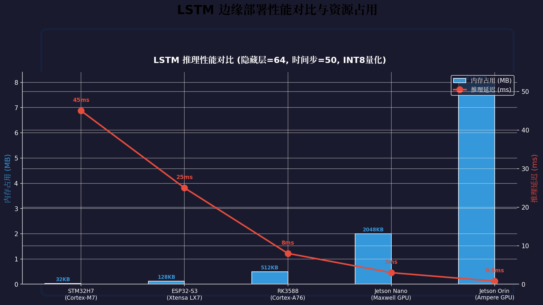
图6：LSTM边缘部署性能对比与资源占用
测试配置：输入维度=6，隐藏层=64，时间步=50，INT8量化，结构化剪枝（稀疏度50%）

平台	处理器	内存占用	推理延迟	功耗	适用场景
STM32H7	Cortex-M7 @480MHz	32KB	45ms	~100mW	单传感器预测
ESP32-S3	Xtensa LX7 @240MHz	128KB	25ms	~240mW	物联网节点
RK3588	Cortex-A76 @2.4GHz	512KB	8ms	~2W	边缘网关
Jetson Nano	Maxwell 128 CUDA	2MB	3ms	~5W	多路视频分析
Jetson Orin	Ampere 2048 CUDA	8MB	0.8ms	~15W	工业AI服务器

6.2 选型建议

资源受限场景（<256KB RAM）：

• 使用STM32H7或ESP32-S3
• 隐藏层限制在16-32
• 时间步限制在20-50
• 必须INT8量化

中等算力场景（256KB-2MB RAM）：

• 使用RK3588或类似ARM SoC
• 隐藏层可达64-128
• 支持FP16或INT8
• 可运行轻量级多任务

高算力场景（>2MB RAM）：

• 使用Jetson系列
• 支持多层LSTM堆叠
• 可运行注意力机制变体
• 支持模型并行

---

七、工业预测维护应用实例

7.1 系统架构

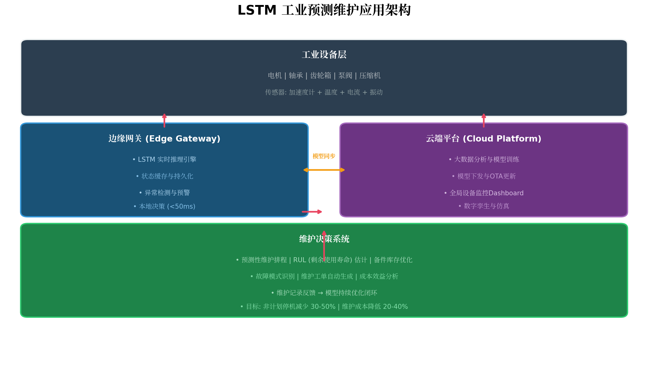
图7：LSTM工业预测维护应用架构

应用场景：旋转机械（电机、轴承、齿轮箱）的振动信号预测维护。

数据采集：

• 三轴加速度计：采样率10kHz，分析频带0-5kHz
• 温度传感器：采样率1Hz
• 电流传感器：采样率1kHz

特征工程：

• 时域特征：RMS、峰值、峰度、偏度
• 频域特征：FFT主频能量、包络谱
• 特征降维：6维输入向量（RMS、温度、电流、频带1能量、频带2能量、频带3能量）

LSTM模型配置：

• 输入维度：6
• 隐藏层：64
• 时间步：100（10秒历史窗口）
• 输出：RUL（剩余使用寿命，小时级）

状态缓存设计：

• SRAM：保存当前 $h_t$ 和 $C_t$（64×2×4B = 512B）
• Flash：每10分钟持久化一次，磨损均衡设计寿命>10年

7.2 推理流水线代码

// 工业预测维护主循环
void predictive_maintenance_loop() {
    static LSTM_StateBuffer lstm_state;
    static float sensor_buffer[FEATURE_DIM];
    static float history_window[TIME_STEPS][FEATURE_DIM];
    static int window_idx = 0;
    
    // 初始化 (仅首次运行)
    if (!lstm_state.initialized) {
        lstm_state_init(&lstm_state, HIDDEN_SIZE);
        lstm_state_restore(&lstm_state, FLASH_STATE_ADDR);
        lstm_state.initialized = 1;
    }
    
    while (1) {
        // 1. 传感器数据采集 (100ms周期)
        read_sensors(sensor_buffer);
        
        // 2. 特征提取与归一化
        extract_features(sensor_buffer, &history_window[window_idx]);
        normalize_features(&history_window[window_idx]);
        
        window_idx = (window_idx + 1) % TIME_STEPS;
        
        // 3. 每10个采样点执行一次推理 (1秒)
        if (window_idx % 10 == 0) {
            float* cell_state, *hidden_state;
            lstm_state_read(&lstm_state, &cell_state, &hidden_state);
            
            // 执行LSTM推理 (100个时间步)
            float predicted_rul = 0.0f;
            for (int t = 0; t < TIME_STEPS; t++) {
                int idx = (window_idx + t) % TIME_STEPS;
                lstm_int8_step(history_window[idx], hidden_state, cell_state, ...);
            }
            
            // 全连接层输出RUL
            predicted_rul = fc_forward(hidden_state);
            
            // 4. 状态更新
            lstm_state_write(&lstm_state, cell_state, hidden_state);
            
            // 5. 异常检测与决策
            if (predicted_rul < RUL_WARNING_THRESHOLD) {
                trigger_warning(predicted_rul);
            }
            if (predicted_rul < RUL_CRITICAL_THRESHOLD) {
                trigger_alarm();
                schedule_maintenance();
            }
            
            // 6. 定期持久化 (每10分钟)
            static int persist_counter = 0;
            if (++persist_counter >= 600) {  // 600秒 = 10分钟
                lstm_state_persist(&lstm_state, FLASH_STATE_ADDR);
                persist_counter = 0;
            }
        }
        
        delay_ms(100);  // 100ms采样周期
    }
}

---

八、总结与展望

本文系统探讨了LSTM在边缘设备上的轻量化实现与优化，核心结论：

优化维度	关键技术	效果
状态缓存	双缓冲 + Flash持久化 + 磨损均衡	掉电保护，状态连续性
量化压缩	INT8对称量化 + 查找表近似	内存减少75%，延迟降低60%
模型压缩	结构化剪枝 + 知识蒸馏	参数量减少50-90%
算子融合	4门合并GEMM + 激活内联	减少70%内存访问
内存优化	原地计算 + 交错布局	消除中间分配，缓存命中率提升4x

未来方向：

1. TinyLSTM：针对MCU的极致优化，隐藏层<16，支持8位量化
2. 神经架构搜索（NAS）：自动搜索适合边缘设备的LSTM变体
3. 联邦学习：边缘设备协同训练，保护数据隐私
4. Transformer时序模型：探索Attention机制在边缘的可行性
5. 存内计算（PIM）：利用ReRAM等新型存储器实现原位计算

---

转载自：https://blog.csdn.net/u014727709/article/details/162674923
欢迎 👍点赞✍评论⭐收藏，欢迎指正