第【12】期--基于朗博信道的VLC信道仿真与可视化分析--maltab完整代码
文章目录
摘要
可见光通信(Visible Light Communication, VLC)利用LED灯同时实现照明和数据传输,近年来在室内定位、物联网、短距离无线通信等领域备受关注。本文通过MATLAB完整仿真了一个典型的室内VLC系统,涵盖房间几何建模、朗伯辐射信道计算、接收功率分布可视化等核心环节。所有代码均已注释并提供清晰的图形输出,适合初学者快速上手,也便于研究者调整参数进行扩展分析。
1 背景
随着无线通信设备数量的爆炸式增长,传统射频(RF)通信频段日益拥挤,频谱资源紧张、干扰严重以及电磁敏感环境(如医院、飞机舱)的使用限制等问题逐渐凸显。可见光通信(Visible Light Communication, VLC) 作为一种新兴的无线通信技术,利用发光二极管(LED)高速明暗变化的特性同时实现照明与数据传输,被认为是缓解RF频谱压力的有力候选方案。
VLC 具有多项独特优势:无需申请专用频谱(可见光波段不受管制)、无电磁辐射(可在医疗设备附近安全使用)、天然抗电磁干扰、以及利用现有照明基础设施即可构建通信网络。室内场景是 VLC 最典型的应用环境——办公室、商场、家庭中的 LED 灯具既能照明,又可作为无线接入点,为手机、笔记本电脑或物联网传感器提供高速数据传输。
然而,VLC 的性能高度依赖于信道特性:LED 的朗伯辐射模式、接收机的视场角(FOV)、房间的几何尺寸、墙壁反射以及障碍物遮挡都会显著影响接收功率和覆盖均匀性。因此,在部署实际系统之前,建立精确的信道仿真模型至关重要。通过仿真可以快速评估不同布局和参数下的功率分布、信噪比、误码率等关键指标,为硬件设计和网络规划提供指导。
2 仿真设置
在室内环境中,可见光信号会因受到墙体、家具和人等的遮挡产生反射与散射,因此, VLC 通信链路主要包括视距链路(Line of Sight, LoS)和非视距链路(NonLine of Sight, NLoS)。据现有的文献表明,受限于 LED 光源的半功率角和传播损耗, LoS 链路的接收信号强度占接收器总接收强度的 95.16%,且至少比最强
的 NLoS 链路的信号强度高 7dB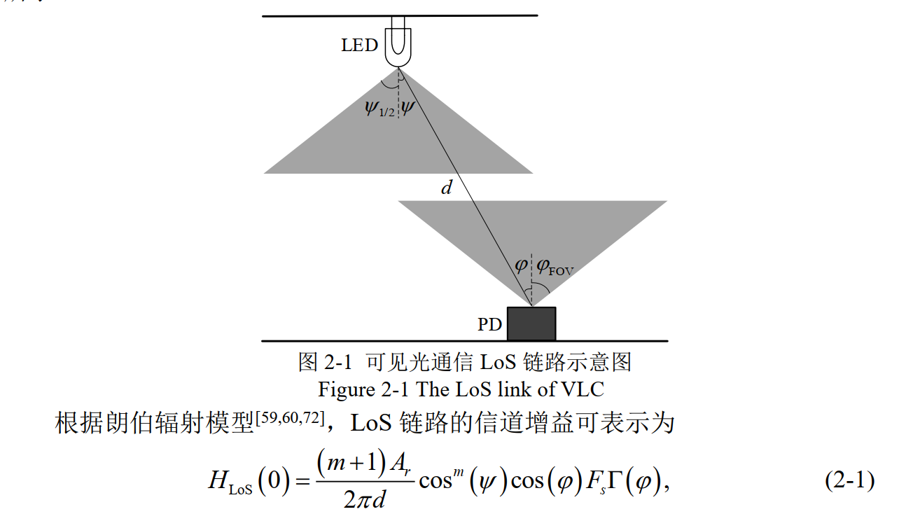
- 优点:形式简单,计算高效:解析表达式,适合大规模网格仿真。广泛使用:绝大多数商用照明LED符合朗伯辐射特性
- 缺点:理想化假设:实际LED可能有微小偏离,尤其在大角度时;不包含反射:仅描述发射机直接辐射,反射路径需额外建模;仅适用于远场:在非常近的距离(厘米级)可能不精确
📊 VLC 系统仿真参数总表
| 类别 | 参数名称 | 数值 | 单位 |
|---|---|---|---|
| 房间几何 | 房间长度(X 轴) | 4.0 | 米 |
| 房间几何 | 房间宽度(Y 轴) | 4.0 | 米 |
| 房间几何 | 房间高度(Z 轴) | 3.0 | 米 |
| 发射机 | 发射机位置 X 坐标 | 0 | 米 |
| 发射机 | 发射机位置 Y 坐标 | 0 | 米 |
| 发射机 | 发射机位置 Z 坐标 | 3 | 米 |
| 发射机 | 发射光功率 | 20 | 瓦 |
| 发射机 | 半功率角 | 70 | 度 |
| 发射机 | 朗伯辐射阶数 | 约 0.96 | 无量纲 |
| 接收机 | 接收机位置 X 坐标 | 1 | 米 |
| 接收机 | 接收机位置 Y 坐标 | 1 | 米 |
| 接收机 | 接收机位置 Z 坐标 | 0.85 | 米 |
| 接收机 | 有效探测面积 | 0.0001 | 平方米 |
| 接收机 | 有效探测面积 | 1 | 平方厘米 |
| 接收机 | 视场角(全角) | 60 | 度 |
| 接收机 | 光滤波器增益 | 1 | 无量纲 |
| 接收机 | 透镜折射率 | 1.5 | 无量纲 |
| 接收机 | 聚光器增益 | 约 3.0 | 无量纲 |
| 仿真网格 | 接收平面高度 | 0.85 | 米 |
| 仿真网格 | 网格分辨率 | 0.05 | 米 |
| 仿真网格 | X 轴范围 | -2 到 2 | 米 |
| 仿真网格 | Y 轴范围 | -2 到 2 | 米 |
| 仿真网格 | 网格点总数 | 6561 | 个 |
| 信道与链路 | 发射机到接收机直线距离 | 约 2.47 | 米 |
仿真代码:
clear; clc; close all;
set(0, 'DefaultAxesFontName', 'Times New Roman');
set(0, 'DefaultTextFontName', 'Times New Roman');
set(0, 'DefaultAxesFontSize', 10);
set(0, 'DefaultTextFontSize', 10);
%% ===== 房间参数 =====
lx = 4; % 长度(X 轴),单位:米
ly = 4; % 宽度(Y 轴),单位:米
lz = 3; % 高度(Z 轴),单位:米
%% ===== 位置坐标 =====
Tx_pos = [0, 0, lz]; % LED 位于天花板中心(x=0, y=0, z=3m)
Rx_pos = [1, 1, 0.85]; % 探测器位于桌面(x=1m, y=1m, z=0.85m)
%% ===== 系统参数 =====
theta_half = 70; % 半功率角(度)
m = -log10(2)/log10(cosd(theta_half)); % 朗伯辐射阶数
P_tx = 20; % LED 发射光功率(瓦)
% 光电探测器参数
A_det = 1e-4; % 有效接收面积(平方米)
FOV_deg = 60; % 视场角(度)
FOV_rad = deg2rad(FOV_deg);
T_s = 1; % 光滤波器增益
n_lens = 1.5; % 透镜折射率
G_con = (n_lens^2)/(sin(FOV_rad)^2); % 聚光器增益
fprintf('\n╔══════════════════════════════════════════════════════════════╗\n');
fprintf('║ VLC 系统 - 完整仿真 ║\n');
fprintf('╚══════════════════════════════════════════════════════════════╝\n');
%% ===== 定义接收平面网格 =====
resolucao = 0.05; % 网格分辨率(米)
x = -lx/2 : resolucao : lx/2;
y = -ly/2 : resolucao : ly/2;
[X_grid, Y_grid] = meshgrid(x, y);
Nx = length(x);
Ny = length(y);
fprintf('网格:%d x %d 个点(分辨率 %.2f 米)\n', Nx, Ny, resolucao);
%% ===== 信道计算 =====
% 三维距离
D_los = sqrt((X_grid - Tx_pos(1)).^2 + (Y_grid - Tx_pos(2)).^2 + (Rx_pos(3) - Tx_pos(3)).^2);
cos_angle = abs(Rx_pos(3) - Tx_pos(3)) ./ D_los;
% 直射(LOS)信道增益
H_los = ((m+1) * A_det ./ (2 * pi * D_los.^2)) .* (cos_angle.^(m+1));
H_los(cos_angle < cosd(FOV_deg)) = 0;
% 非视距反射(简化模型)
H_nlos = H_los * 0.05;
H_total = H_los + H_nlos;
% 接收光功率
P_rec = P_tx * H_total * T_s * G_con;
P_rec_dBm = 10 * log10(P_rec * 1000);
% 接收机位置对应的索引
[~, idx_rx_x] = min(abs(x - Rx_pos(1)));
[~, idx_rx_y] = min(abs(y - Rx_pos(2)));
P_rec_rx = P_rec(idx_rx_y, idx_rx_x);
P_rec_rx_dBm = P_rec_dBm(idx_rx_y, idx_rx_x);
dist_tx_rx = sqrt((Rx_pos(1)-Tx_pos(1))^2 + (Rx_pos(2)-Tx_pos(2))^2 + (Rx_pos(3)-Tx_pos(3))^2);
fprintf('接收机处接收功率:%.2f dBm(%.2f μW)\n', P_rec_rx_dBm, P_rec_rx*1e6);
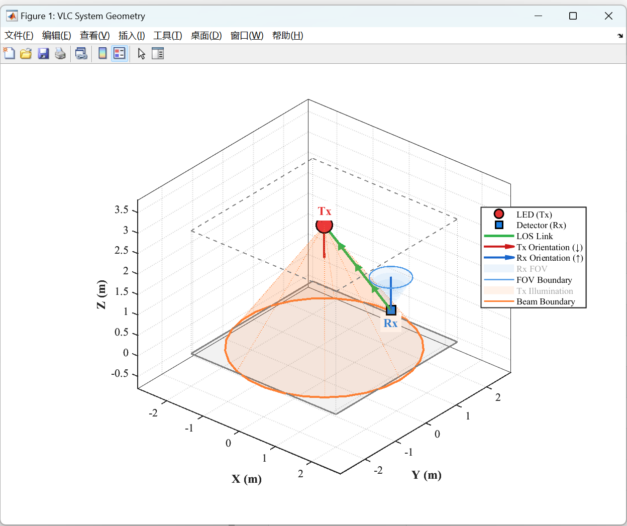
%% ============================================
% 图1:VLC 系统几何结构(3D)
% ============================================
% 配色方案
cores = struct();
cores.parede = [0.5, 0.5, 0.5];
cores.tx = [0.9, 0.2, 0.2];
cores.tx_glow = [1, 0.3, 0.3];
cores.rx = [0.1, 0.5, 0.9];
cores.link = [0.2, 0.7, 0.3];
cores.seta_tx = [0.8, 0.1, 0.1];
cores.seta_rx = [0.1, 0.4, 0.8];
cores.fov = [0.3, 0.6, 0.9];
cores.led_beam = [1, 0.5, 0.2];
fig1 = figure('Name', 'VLC System Geometry', ...
'Position', [50, 500, 1000, 700], ...
'Color', 'white');
hold on; grid on; axis equal;
xlim([-lx/2-0.8, lx/2+0.8]);
ylim([-ly/2-0.8, ly/2+0.8]);
zlim([-0.8, lz+0.8]);
view(40, 30);
% 地面
[X_floor, Y_floor] = meshgrid(linspace(-lx/2, lx/2, 50), linspace(-ly/2, ly/2, 50));
surf(X_floor, Y_floor, zeros(size(X_floor)), 'FaceAlpha', 0.1, 'EdgeColor', 'none', 'FaceColor', cores.parede);
% 房间棱边
plot3([-lx/2, lx/2], [-ly/2, -ly/2], [0, 0], 'Color', cores.parede, 'LineWidth', 1.5);
plot3([-lx/2, lx/2], [ly/2, ly/2], [0, 0], 'Color', cores.parede, 'LineWidth', 1.5);
plot3([-lx/2, -lx/2], [-ly/2, ly/2], [0, 0], 'Color', cores.parede, 'LineWidth', 1.5);
plot3([lx/2, lx/2], [-ly/2, ly/2], [0, 0], 'Color', cores.parede, 'LineWidth', 1.5);
plot3([-lx/2, lx/2], [-ly/2, -ly/2], [lz, lz], 'Color', cores.parede, 'LineWidth', 1, 'LineStyle', '--');
plot3([-lx/2, lx/2], [ly/2, ly/2], [lz, lz], 'Color', cores.parede, 'LineWidth', 1, 'LineStyle', '--');
plot3([-lx/2, -lx/2], [-ly/2, ly/2], [lz, lz], 'Color', cores.parede, 'LineWidth', 1, 'LineStyle', '--');
plot3([lx/2, lx/2], [-ly/2, ly/2], [lz, lz], 'Color', cores.parede, 'LineWidth', 1, 'LineStyle', '--');
% 竖直棱线(虚线)
plot3([-lx/2, -lx/2], [-ly/2, -ly/2], [0, lz], 'Color', cores.parede, 'LineWidth', 0.5, 'LineStyle', ':');
plot3([lx/2, lx/2], [-ly/2, -ly/2], [0, lz], 'Color', cores.parede, 'LineWidth', 0.5, 'LineStyle', ':');
plot3([-lx/2, -lx/2], [ly/2, ly/2], [0, lz], 'Color', cores.parede, 'LineWidth', 0.5, 'LineStyle', ':');
plot3([lx/2, lx/2], [ly/2, ly/2], [0, lz], 'Color', cores.parede, 'LineWidth', 0.5, 'LineStyle', ':');
% LED 发射机
[Xs, Ys, Zs] = sphere(20);
surf(Xs*0.18 + Tx_pos(1), Ys*0.18 + Tx_pos(2), Zs*0.18 + Tx_pos(3), ...
'FaceAlpha', 0.2, 'EdgeColor', 'none', 'FaceColor', cores.tx_glow);
h_tx = plot3(Tx_pos(1), Tx_pos(2), Tx_pos(3), 'o', 'MarkerSize', 16, ...
'MarkerFaceColor', cores.tx, 'MarkerEdgeColor', 'k', 'LineWidth', 1.5);
text(Tx_pos(1), Tx_pos(2), Tx_pos(3)+0.35, 'Tx', 'Color', cores.tx, 'FontSize', 12, 'FontWeight', 'bold', ...
'HorizontalAlignment', 'center', 'BackgroundColor', 'white');
% 探测器
h_rx = plot3(Rx_pos(1), Rx_pos(2), Rx_pos(3), 's', 'MarkerSize', 12, ...
'MarkerFaceColor', cores.rx, 'MarkerEdgeColor', 'k', 'LineWidth', 1.5);
text(Rx_pos(1), Rx_pos(2), Rx_pos(3)-0.3, 'Rx', 'Color', cores.rx, 'FontSize', 12, 'FontWeight', 'bold', ...
'HorizontalAlignment', 'center', 'BackgroundColor', 'white');
% 直射链路(LOS)
h_link = plot3([Tx_pos(1), Rx_pos(1)], [Tx_pos(2), Rx_pos(2)], [Tx_pos(3), Rx_pos(3)], ...
'Color', cores.link, 'LineWidth', 2.5, 'LineStyle', '-');
t = 0.25:0.25:0.75;
for tt = t
x_int = Tx_pos(1) + tt*(Rx_pos(1)-Tx_pos(1));
y_int = Tx_pos(2) + tt*(Rx_pos(2)-Tx_pos(2));
z_int = Tx_pos(3) + tt*(Rx_pos(3)-Tx_pos(3));
plot3(x_int, y_int, z_int, '>', 'Color', cores.link, 'MarkerSize', 7, 'MarkerFaceColor', cores.link);
end
% 方向箭头
h_arrow_tx = quiver3(Tx_pos(1), Tx_pos(2), Tx_pos(3), 0, 0, -0.8, 'Color', cores.seta_tx, ...
'LineWidth', 2, 'MaxHeadSize', 0.5, 'AutoScale', 'off');
h_arrow_rx = quiver3(Rx_pos(1), Rx_pos(2), Rx_pos(3), 0, 0, 0.8, 'Color', cores.seta_rx, ...
'LineWidth', 2, 'MaxHeadSize', 0.5, 'AutoScale', 'off');
% 接收机视场(FOV)锥体
angulo_fov_rad = deg2rad(FOV_deg);
altura_cone_fov = 0.8;
raio_cone_fov = altura_cone_fov * tan(angulo_fov_rad/2);
theta_c = linspace(0, 2*pi, 30);
x_cone_fov = Rx_pos(1) + raio_cone_fov * cos(theta_c);
y_cone_fov = Rx_pos(2) + raio_cone_fov * sin(theta_c);
z_cone_fov_top = ones(size(theta_c)) * (Rx_pos(3) + altura_cone_fov);
for altura = linspace(0, altura_cone_fov, 8)
raio_atual = altura * tan(angulo_fov_rad/2);
x_atual = Rx_pos(1) + raio_atual * cos(theta_c);
y_atual = Rx_pos(2) + raio_atual * sin(theta_c);
z_atual = ones(size(theta_c)) * (Rx_pos(3) + altura);
patch(x_atual, y_atual, z_atual, cores.fov, 'FaceAlpha', 0.08, 'EdgeColor', 'none');
end
h_fov_edge = plot3(x_cone_fov, y_cone_fov, z_cone_fov_top, 'Color', cores.fov, 'LineWidth', 1.2, 'LineStyle', '-');
% LED 照明锥体
angulo_led_rad = deg2rad(theta_half);
raio_led_base = lz * tan(angulo_led_rad/2);
[Theta_grid, R_grid] = meshgrid(theta_c, linspace(0, 1, 20));
X_cone_beam = Tx_pos(1) + R_grid * raio_led_base .* cos(Theta_grid);
Y_cone_beam = Tx_pos(2) + R_grid * raio_led_base .* sin(Theta_grid);
Z_cone_beam = lz * (1 - R_grid);
surf(X_cone_beam, Y_cone_beam, Z_cone_beam, 'FaceColor', cores.led_beam, 'FaceAlpha', 0.12, 'EdgeColor', 'none');
x_led_base = Tx_pos(1) + raio_led_base * cos(theta_c);
y_led_base = Tx_pos(2) + raio_led_base * sin(theta_c);
h_beam_edge = plot3(x_led_base, y_led_base, zeros(size(theta_c)), 'Color', cores.led_beam, 'LineWidth', 1.5, 'LineStyle', '-');
plot3(x_led_base, y_led_base, zeros(size(theta_c)), 'Color', cores.led_beam, 'LineWidth', 2, 'LineStyle', '-');
for i = 1:5:length(theta_c)
plot3([Tx_pos(1), x_led_base(i)], [Tx_pos(2), y_led_base(i)], [lz, 0], ...
'Color', cores.led_beam, 'LineWidth', 0.8, 'LineStyle', ':');
end
% 坐标轴标签
xlabel('X (m)', 'FontSize', 12, 'FontWeight', 'bold');
ylabel('Y (m)', 'FontSize', 12, 'FontWeight', 'bold');
zlabel('Z (m)', 'FontSize', 12, 'FontWeight', 'bold');
% 图例(使用不可见对象辅助)
h_fov_legend = patch('XData', [0 1 1 0], 'YData', [0 0 1 1], 'ZData', [0 0 0 0], ...
'FaceColor', cores.fov, 'FaceAlpha', 0.3, 'EdgeColor', 'none', 'Visible', 'off');
h_beam_legend = patch('XData', [0 1 1 0], 'YData', [0 0 1 1], 'ZData', [0 0 0 0], ...
'FaceColor', cores.led_beam, 'FaceAlpha', 0.3, 'EdgeColor', 'none', 'Visible', 'off');
legend([h_tx, h_rx, h_link, h_arrow_tx, h_arrow_rx, h_fov_legend, h_fov_edge, h_beam_legend, h_beam_edge], ...
{'LED (Tx)', 'Detector (Rx)', 'LOS Link', 'Tx Orientation (↓)', 'Rx Orientation (↑)', ...
'Rx FOV', 'FOV Boundary', 'Tx Illumination', 'Beam Boundary'}, ...
'Location', 'eastoutside', 'FontSize', 9, 'Box', 'on', 'Color', 'white');
set(gca, 'FontSize', 11, 'LineWidth', 1, 'GridAlpha', 0.15, 'GridLineStyle', ':', 'Box', 'on', 'TickDir', 'out');
hold off;
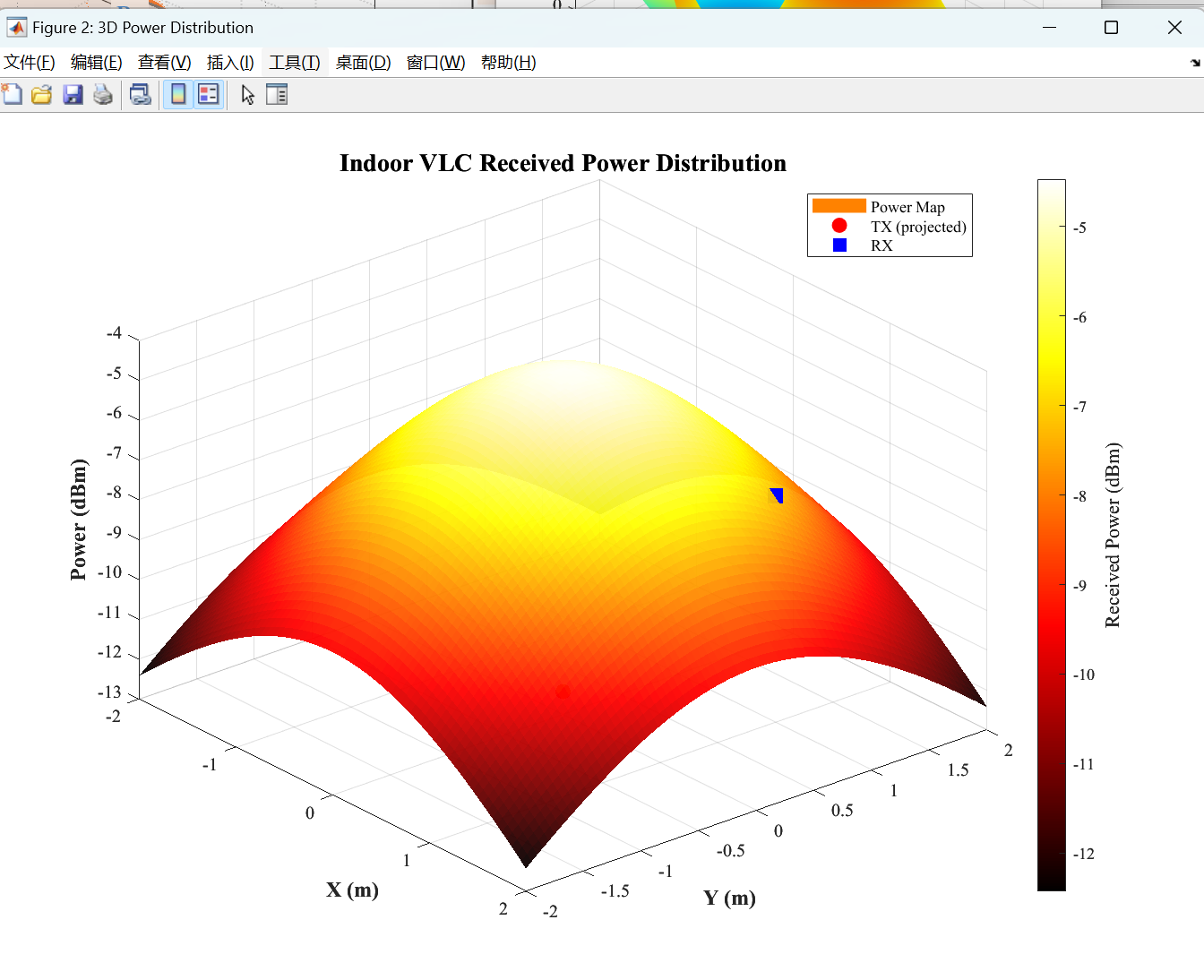
%% ============================================
% 图2:三维功率分布图
% ============================================
fig2 = figure('Name', '3D Power Distribution', 'Position', [50, 50, 900, 650], 'Color', 'white');
surf(X_grid, Y_grid, P_rec_dBm, 'EdgeColor', 'none', 'FaceAlpha', 0.95);
colormap('hot');
cbar = colorbar('eastoutside');
cbar.Label.String = 'Received Power (dBm)';
cbar.Label.FontSize = 11;
title('Indoor VLC Received Power Distribution', 'FontSize', 14, 'FontWeight', 'bold');
xlabel('X (m)', 'FontSize', 12, 'FontWeight', 'bold');
ylabel('Y (m)', 'FontSize', 12, 'FontWeight', 'bold');
zlabel('Power (dBm)', 'FontSize', 12, 'FontWeight', 'bold');
grid on; view(50, 35);
hold on;
plot3(Tx_pos(1), Tx_pos(2), min(P_rec_dBm(:)), 'ro', 'MarkerSize', 8, 'MarkerFaceColor', 'r');
plot3(Rx_pos(1), Rx_pos(2), P_rec_dBm(idx_rx_y, idx_rx_x), 'bs', 'MarkerSize', 10, 'MarkerFaceColor', 'b');
legend('Power Map', 'TX (projected)', 'RX', 'Location', 'northeast');
hold off;
%% ============================================
% 图3:功率剖面图(沿 y=0 切割)
% =============================================
fig3 = figure('Name', 'Power Profile', 'Position', [980, 50, 800, 500], 'Color', 'white');
[~, idx_y_zero] = min(abs(y - 0));
perfil_total = P_rec_dBm(idx_y_zero, :);
perfil_los = 10*log10(P_tx * H_los(idx_y_zero, :) * T_s * G_con * 1000);
perfil_nlos = 10*log10(P_tx * H_nlos(idx_y_zero, :) * T_s * G_con * 1000);
hold on;
fill([x, fliplr(x)], [perfil_total, fliplr(perfil_total)], [0.9, 0.7, 0.4], 'FaceAlpha', 0.15, 'EdgeColor', 'none');
p3 = plot(x, perfil_total, '-', 'Color', [0.2, 0.3, 0.4], 'LineWidth', 3);
p1 = plot(x, perfil_los, '-', 'Color', [0.2, 0.7, 0.3], 'LineWidth', 2);
p2 = plot(x, perfil_nlos, '--', 'Color', [0.9, 0.4, 0.2], 'LineWidth', 2);
xline(Tx_pos(1), '--', 'Color', [0.9, 0.2, 0.2], 'LineWidth', 1.5);
xline(Rx_pos(1), '--', 'Color', [0.1, 0.5, 0.9], 'LineWidth', 1.5);
[peak_val, peak_idx] = max(perfil_total);
plot(x(peak_idx), peak_val, '^', 'MarkerSize', 10, 'MarkerFaceColor', [0.9, 0.6, 0.2], 'MarkerEdgeColor', 'k');
xlim([-2.2, 2.2]); ylim([-14, 12]);
grid on;
xlabel('X (m)', 'FontSize', 12, 'FontWeight', 'bold');
ylabel('Power (dBm)', 'FontSize', 12, 'FontWeight', 'bold');
title('Power Profile along X-axis (y = 0)', 'FontSize', 13, 'FontWeight', 'bold');
legend([p3, p1, p2], {'Total Power', 'LOS Component', 'NLOS Component'}, ...
'Location', 'southwest', 'FontSize', 10, 'Box', 'on');
hold off;
%% ============================================
% 图4:系统信息面板
% ============================================
fig4 = figure('Name', 'System Information', 'Position', [850, 550, 450, 500], 'Color', 'white');
axis off;
info_text = {
'╔══════════════════════════════════════╗';
'║ VLC SYSTEM SUMMARY ║';
'╚══════════════════════════════════════╝';
' ';
'🔴 TRANSMITTER (LED)';
sprintf(' Position: [%.2f, %.2f, %.2f] m', Tx_pos(1), Tx_pos(2), Tx_pos(3));
sprintf(' Optical power: %.1f W', P_tx);
sprintf(' Half-power angle: %.1f°', theta_half);
sprintf(' Lambertian order: %.2f', m);
' ';
'🔵 RECEIVER (Detector)';
sprintf(' Position: [%.2f, %.2f, %.2f] m', Rx_pos(1), Rx_pos(2), Rx_pos(3));
sprintf(' Effective area: %.2f cm²', A_det*1e4);
sprintf(' FOV: %.1f°', FOV_deg);
sprintf(' Concentrator gain: %.2f', G_con);
' ';
'🟢 LINK';
sprintf(' TX-RX distance: %.2f m', dist_tx_rx);
sprintf(' Received power: %.2f dBm', P_rec_rx_dBm);
sprintf(' Received power: %.2f μW', P_rec_rx*1e6);
' ';
'📊 STATISTICS';
sprintf(' Maximum power: %.2f dBm', max(P_rec_dBm(:)));
sprintf(' Mean power: %.2f dBm', mean(P_rec_dBm(:)));
sprintf(' Minimum power: %.2f dBm', min(P_rec_dBm(:)));
};
text(0.05, 0.95, info_text, 'FontName', 'Courier New', 'FontSize', 10, 'VerticalAlignment', 'top');
title('VLC System Summary', 'FontSize', 14, 'FontWeight', 'bold');
%% ===== 结束信息 =====
fprintf('\n╔══════════════════════════════════════════════════════════════╗\n');
fprintf('║ ✅ 仿真完成 ║\n');
fprintf('╚══════════════════════════════════════════════════════════════╝\n');
fprintf('\n📊 已生成图形:\n');
fprintf(' ■ Figure 1: VLC System 3D Geometry\n');
fprintf(' ■ Figure 2: 3D Power Distribution Map\n');
fprintf(' ■ Figure 3: Power Profile (y=0 cut)\n');
fprintf(' ■ Figure 4: System Information Panel\n');
% 注意:以下动画生成部分与 VLC 仿真无关,为独立示例代码,保留原样但注释已中文化
% 设置三维视角并显示网格
view(3);
grid on;
% 定义 GIF 文件名
num_frames = 30; % 30 帧
filename = 'src/canal_vlc_3d.gif';
% 若目录不存在则创建
if ~exist(fileparts(filename), 'dir')
mkdir(fileparts(filename));
end
% 循环生成 GIF
for i = 1:num_frames
% 生成示例数据(随时间变化的正弦曲面)
x = linspace(-3, 3, 100);
y = linspace(-3, 3, 100);
[X, Y] = meshgrid(x, y);
Z = sin(X) .* cos(Y + i/5); % 相位随帧变化
% 绘制当前帧
surf(X, Y, Z);
shading interp
colormap jet
view(45, 30)
axis tight
% 捕获当前图形
frame = getframe(gcf);
im = frame2im(frame);
[imind, cm] = rgb2ind(im, 256);
% 写入 GIF 文件
if i == 1
imwrite(imind, cm, filename, 'gif', 'Loopcount', inf, 'DelayTime', 0.1);
else
imwrite(imind, cm, filename, 'gif', 'WriteMode', 'append', 'DelayTime', 0.1);
end
end
disp(['GIF saved to: ' filename]);
后续优化建议:
多LED布局:将单灯改为4盏或9盏阵列,研究照明均匀性与通信覆盖的折衷。
移动接收机:动态改变Rx位置并记录功率变化,生成轨迹上的功率曲线。
阻挡物模拟:引入人体或家具遮挡的NLOS建模,观察LOS中断时NLOS能否维持基本通信。

智能硬件社区聚焦AI智能硬件技术生态,汇聚嵌入式AI、物联网硬件开发者,打造交流分享平台,同步全国赛事资讯、开展 OPC 核心人才招募,助力技术落地与开发者成长。
更多推荐
 5
5 0
0- 0


 已为社区贡献1条内容

所有评论(0)